Note
Click here to download the full example code
Studying realistic bosonic qubits using the bosonic backend
Note
This tutorial is third in a series on the bosonic backend. For an introduction
to the backend, see part 1. To learn about
how the backend can be used to sample non-Gaussian states, see
part 2. These tutorials accompany
our research paper [1].
In a previous tutorial, we briefly introduced
Gottesman-Kitaev-Preskill (GKP) states [2] as an example of
non-Gaussian states which can be simulated using the bosonic
backend. Here, we use the bosonic backend to take a deep dive into
the advantages of using GKP states as a means for encoding a qubit in a
photonic mode. GKP qubits have a key property that we will
explore in this tutorial: a universal set of qubit gates and measurements can be
applied using the already-familiar Gaussian gates and measurements from
previous tutorials.
After providing more intuition for what ideal and practical GKP states
look like in phase space, we will show how to apply qubit gates and
measurements, and how such operations perform under realistic, noisy
conditions. While some of these simulations have been performed before,
many of these, especially the two-qubit Clifford gates and the T-gate
teleportation circuits have eluded simulation because of their computational
cost. The bosonic backend brings these simulations to within our reach.
We assume that readers of this tutorial have some familiarity with phase space methods like the Wigner function and basic CV gates, as well as basic qubit gates.
GKP states as qubits
In an ideal world
For the GKP encoding, the Wigner function of the ideal qubit \(|0\rangle_{\rm gkp}\) state consists of a linear combination of Dirac delta functions centred at half-integer multiples of \(\sqrt{\pi\hbar}\) in phase space [2]:
The GKP qubit \(|1\rangle_{\rm gkp}\) state can be obtained by shifting the \(|0\rangle_{\rm gkp}\) state by \(\sqrt{\pi\hbar}\) in the position quadrature [2].
Below is a visualization of the ideal \(|0\rangle_{\rm gkp}\) and \(|1\rangle_{\rm gkp}\)
states in phase space using the bosonic backend [3]. Each blue (red) dot
represents a positive (negative) delta function.
# Import relevant libraries
import strawberryfields as sf
import numpy as np
import matplotlib.pyplot as plt
from matplotlib import colors, colorbar

# Set the scale for phase space
sf.hbar = 1
scale = np.sqrt(sf.hbar * np.pi)

# Create a GKP |0> state
prog = sf.Program(1)

with prog.context as q:
    sf.ops.GKP() | q

eng = sf.Engine("bosonic")
gkp_0 = eng.run(prog).state

# Create a GKP |1> state
prog = sf.Program(1)

with prog.context as q:
    sf.ops.GKP() | q
    sf.ops.Xgate(np.sqrt(np.pi * sf.hbar)) | q

eng = sf.Engine("bosonic")
gkp_1 = eng.run(prog).state

# Get the phase space coordinates of the delta functions for the two states
q_coords_0 = gkp_0.means().real[:, 0]
p_coords_0 = gkp_0.means().real[:, 1]
q_coords_1 = gkp_1.means().real[:, 0]
p_coords_1 = gkp_1.means().real[:, 1]

# Determine whether the delta functions are positively or negatively weighted
delta_sign_0 = np.sign(gkp_0.weights().real)
delta_sign_1 = np.sign(gkp_1.weights().real)

# Plot the locations and signs of the deltas
fig,ax = plt.subplots(1, 2)
ax[0].scatter(q_coords_0 / scale,
           p_coords_0 / scale,
           c=delta_sign_0,
           cmap=plt.cm.RdBu, vmin=-1.5, vmax=1.5)
ax[1].scatter(q_coords_1 / scale,
           p_coords_1 / scale,
           c=delta_sign_0,
           cmap=plt.cm.RdBu, vmin=-1.5, vmax=1.5)
for i in range(2):
    ax[i].set_xlim(-3.5, 3.5)
    ax[i].set_ylim(-3.5, 3.5)
    ax[i].set_xlabel(r'$q$ (units of $\sqrt{\pi\hbar}$ )', fontsize=15)
    ax[i].set_aspect("equal")
ax[0].set_title(r'$|0\rangle_{\rm gkp}$ Wigner function', fontsize=15)
ax[1].set_title(r'$|1\rangle_{\rm gkp}$ Wigner function', fontsize=15)
ax[0].set_ylabel(r'$p$ (units of $\sqrt{\pi\hbar}$ )', fontsize=15)
fig.tight_layout()
plt.show()
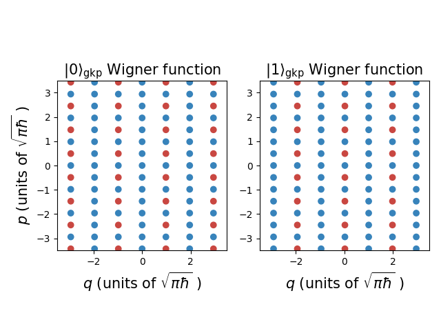
Like standard qubit \(|0\rangle\) and \(|1\rangle\) states, these two states are orthogonal: wherever the \(|0\rangle_{\rm gkp}\) state has a column of delta functions with alternating signs, the \(|1\rangle_{\rm gkp}\) state has a column of all positive delta functions, and vice versa. This results in a zero overlap between the \(|0\rangle_{\rm gkp}\) and \(|1\rangle_{\rm gkp}\) Wigner functions, meaning they are orthogonal.
The Wigner function for a general qubit state
also consists of a weighted linear combination of delta functions at half-integer multiples of \(\sqrt{\pi\hbar}\) in phase space, with the weights depending \(\theta\) and \(\phi\) [4, 1].
One might have already noticed a problem: since their Wigner functions consist of a linear combination of deltas, ideal GKP states have infinite energy, cannot be normalized, and are therefore unphysical!
Let’s get physical
Phyiscal, normalizable and finite-energy GKP states can be constructed by applying a Fock damping operator to the ideal states:
where \(\hat{n}\) is the photon number operator. For any realistic application calling for GKP states, finite-energy GKP states will need to be employed.
Through a mathematical derivation best enjoyed with coffee ☕ and a snack 🍪 [1], we find the effect of the finite-energy operator on the GKP Wigner functions to be as follows:
Each delta function is replaced with a Gaussian function of non-zero variance.
The location of each of these new Gaussian peaks is contracted towards the origin.
The weights of the Gaussians are damped the further the peak is located from the origin.
As we saw in the introductory tutorial, Wigner functions that can be
expressed as a linear combination of Gaussian functions in phase space
are the bread and butter of the bosonic backend. Now we have shown
exactly how GKP states fall neatly into that form.
For these new sets of Gaussian peaks, the variance, the location shift, and the damping of the weights all depend on the finite-energy parameter \(\epsilon\). Let’s visualize how the Wigner function changes as we vary \(\epsilon\):
# Choose some values of epsilon
epsilons = [0.05, 0.1, 0.2, 5]

# Pick a region of phase space to plot
quad = np.linspace(-3.5, 3.5, 200) * scale

wigners = []

for epsilon in epsilons:

    # Create a GKP |0> state
    prog = sf.Program(1)

    with prog.context as q:
        sf.ops.GKP(epsilon=epsilon) | q

    eng = sf.Engine("bosonic")
    gkp = eng.run(prog).state

    # Calculate the Wigner function
    wigner = gkp.wigner(mode=0, xvec=quad, pvec=quad)
    wigners.append(wigner)

# Plot the results
fig, axs = plt.subplots(1, 5, figsize=(16, 4), gridspec_kw={"width_ratios": [1, 1, 1, 1, 0.05]})
cmap = plt.cm.RdBu
cmax = np.real_if_close(np.amax(np.array(wigners)))
norm = colors.Normalize(vmin=-cmax, vmax=cmax)
cb1 = colorbar.ColorbarBase(axs[4], cmap=cmap, norm=norm, orientation="vertical")
for i in range(4):
    axs[i].contourf(
        quad / scale,
        quad / scale,
        wigners[i],
        levels=60,
        cmap=plt.cm.RdBu,
        vmin=-cmax,
        vmax=cmax,
    )
    axs[i].set_title(r'$\epsilon =$'+str(epsilons[i]), fontsize=15)
    axs[i].set_xlabel(r'$q$ (units of $\sqrt{\pi\hbar}$ )', fontsize=15)
axs[0].set_ylabel(r'$p$ (units of $\sqrt{\pi\hbar}$ )', fontsize=15)
cb1.set_label("Wigner function", fontsize=15)
fig.tight_layout()
plt.show()
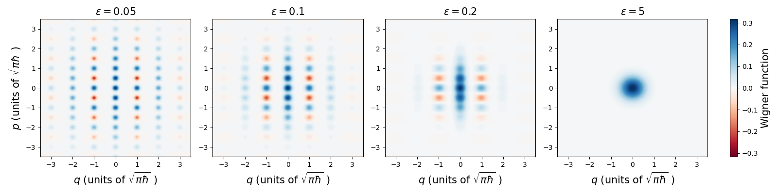
We see that as \(\epsilon\) increases, the variance of each peak grows, the peaks get closer and closer to the origin, and the weights (which govern how large the Wigner function gets) drop exponentially away from the origin. In the limit as \(\epsilon\rightarrow\infty\), the Fock damping gets so strong that all we are left with is the vacuum state, as can be seen in the last plot.
Since the delta spikes are now Gaussians, the \(|0^\epsilon\rangle_{\rm gkp}\) and \(|1^\epsilon\rangle_{\rm gkp}\) states are no longer exactly orthogonal, which will lead to a small but inherent readout error when distinguishing the computational-basis states. As compared to ideal GKP qubits, finite-energy qubits are noisier; consequently, we can refer to this type of imperfection as “finite-energy noise”.
Now that we’ve established that realistic GKP states fall under the
simulation capabilities of the bosonic backend, let’s go through the
set of qubit measurements and gates for a GKP state. We’ll see that the
only resources one needs in addition to GKP states are Gaussian
transformations and measurements [5], which we also know to be easily
simulated using the bosonic backend.
Qubit Pauli measurements: CV homodyne measurements
The first example of correspondence between GKP qubit operations and Gaussian resources are Pauli measurements. For GKP qubits, they can be implemented by performing homodyne measurements and processing the outcomes. The association is:
Pauli |
Homodyne |
|
|---|---|---|
Z |
\(q\) |
|
X |
\(p\) |
|
Y |
\(q-p\) |
The outcomes of these homodyne measurements are rounded or “binned” to the nearest \(n\sqrt{\pi\hbar}\), \(n\in\mathbb{Z}\). Then, the parity of \(n\) is taken to determine the value of the Pauli measurement. Note that the Pauli Y measurements can be achieved by performing a homodyne measurement along \((q - p)/\sqrt{2}\) and rescaling by \(\sqrt{2}\).
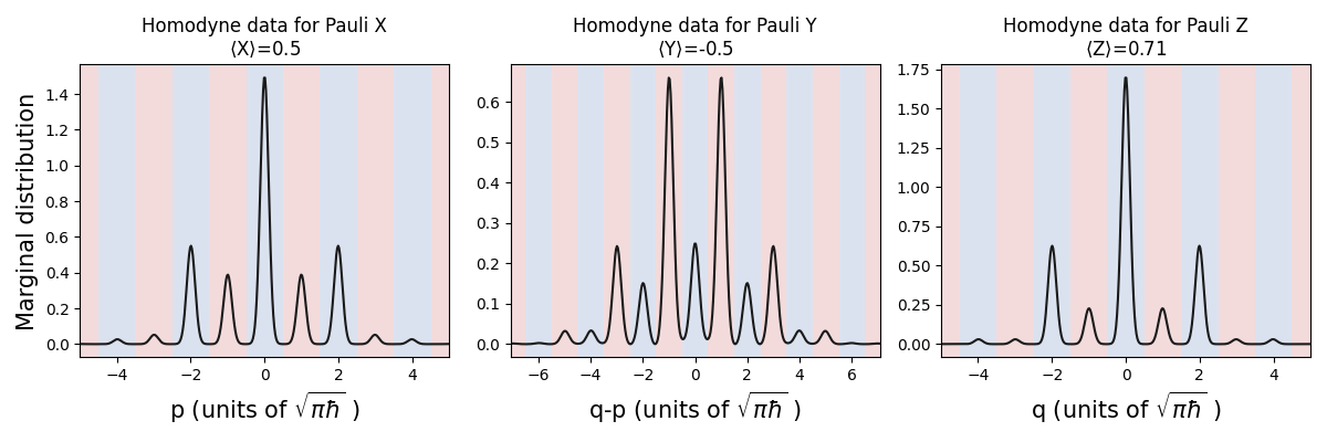
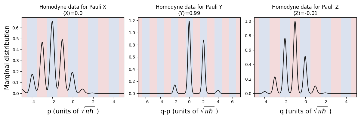
As an example, we look at the marginal distributions of homodyne outcomes for GKP \(|+^\epsilon\rangle_{\rm gkp}\) to confirm Pauli measurements can be performed with homodyne. Alternatively, we could have directly simulated samples like in the last tutorial.
The angles \(\theta,\phi\) that specify the qubit state can be passed to the
sf.ops.GKP() operation via the state parameter.
The homodyne outcomes that fall into blue (red) bins can be interpreted as a Pauli operator eigenvalue measurement with outcome \(+1\) (\(-1\)). The bins can be used to provide the expectation value of each Pauli operator: we integrate the marginal distributions, each multiplied by an appropriate weighting function that changes the sign of the distribution depending on the Pauli operator eigenvalue associated with the bin.
# Create a GKP |+> state
plus = [np.pi / 2, 0]
prog = sf.Program(1)

with prog.context as q:
    sf.ops.GKP(state=plus, epsilon=0.08) | q

eng = sf.Engine("bosonic")
gkp = eng.run(prog).state

def calc_and_plot_marginals(state, mode):
    '''Calculates and plots the p, q-p, and q quadrature marginal
    distributions for a given circuit mode. These can be used to determine
    the Pauli X, Y, and Z outcomes for a GKP qubit.

    Args:
        state (object): a strawberryfields ``BaseBosonicState`` object
        mode (int): index for the circuit mode
    '''
    # Calculate the marginal distributions.
    # The rotation angle in phase space is specified by phi
    marginals = []
    phis = [np.pi / 2, -np.pi / 4, 0]
    quad = np.linspace(-5, 5, 400) * scale
    for phi in phis:
        marginals.append(state.marginal(mode, quad, phi=phi))

    # Plot the results
    paulis = ["X", "Y", "Z"]
    homodynes = ["p", "q-p", "q"]
    expectations = np.zeros(3)

    fig, axs = plt.subplots(1, 3, figsize=(12, 4))
    for i in range(3):
        if i == 1:
            # Rescale the outcomes for Pauli Y
            y_scale = np.sqrt(2 * sf.hbar) / scale
            axs[i].plot(quad * y_scale, marginals[i] / y_scale, 'k-')
            axs[i].set_xlim(quad[0] * y_scale, quad[-1] * y_scale)

            # Calculate Pauli expectation value
            # Blue bins are weighted +1, red bins are weighted -1
            bin_weights = 2 * (((quad * y_scale - 0.5) // 1) % 2) - 1
            integrand = (marginals[i] / y_scale) * bin_weights
            expectations[i] = np.trapz(integrand, quad * y_scale)
        else:
            axs[i].plot(quad / scale, marginals[i] * scale, 'k-')
            axs[i].set_xlim(quad[0] / scale, quad[-1] / scale)

            # Calculate Pauli expectation value
            # Blue bins are weighted +1, red bins are weighted -1
            bin_weights = 2 * (((quad / scale - 0.5) // 1) % 2) - 1
            integrand = (marginals[i] * scale) * bin_weights
            expectations[i] = np.trapz(integrand, quad / scale)

        # Color the qubit bins blue and red
        for j in range(-10, 10):
            axs[i].axvspan((2 * j - 0.5), (2 * j + 0.5), alpha=0.2, facecolor='b')
            axs[i].axvspan((2 * j + 0.5), (2 * j + 1.5), alpha=0.2, facecolor='r')

        axs[i].set_title("Homodyne data for Pauli " + paulis[i] +
                         "\n" + r'$\langle$'+paulis[i]+r'$\rangle$='+
                         str(np.around(expectations[i],2)))
        axs[i].set_xlabel(homodynes[i] + r' (units of $\sqrt{\pi\hbar}$ )', fontsize=15)
    axs[0].set_ylabel("Marginal distribution", fontsize=15)
    fig.tight_layout()
    plt.show()

calc_and_plot_marginals(gkp, 0)
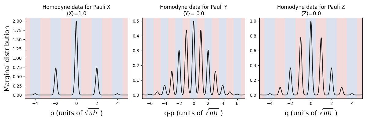
We can see from the \(p\)-homodyne measurement outcomes that the results are mostly within the blue bins, so there will be a high chance of reading out a \(+1\) eigenvalue from a Pauli X measurement, as would be expected for a standard qubit \(|+\rangle\) state.
For the other two homodyne measurements, the peaks of the marginal distributions are effectively evenly distributed between \(+1\) and \(-1\) bins, just like Pauli Y and Z measurements on a standard qubit \(|+\rangle\) state.
One of the strengths of the bosonic backend is the ease of applying
Gaussian transformations to states. For qubits encoded in CV systems, a
major source of noise is loss or dissipation. Let’s see how the
distributions of homodyne outcomes change after we apply the
LossChannel operation:
# Create a GKP |+> state and apply loss
prog = sf.Program(1)

with prog.context as q:
    sf.ops.GKP(state=plus, epsilon=0.08) | q
    sf.ops.LossChannel(0.85) | q

eng = sf.Engine("bosonic")
gkp = eng.run(prog).state

#Calculate and plot marginals
calc_and_plot_marginals(gkp, 0)
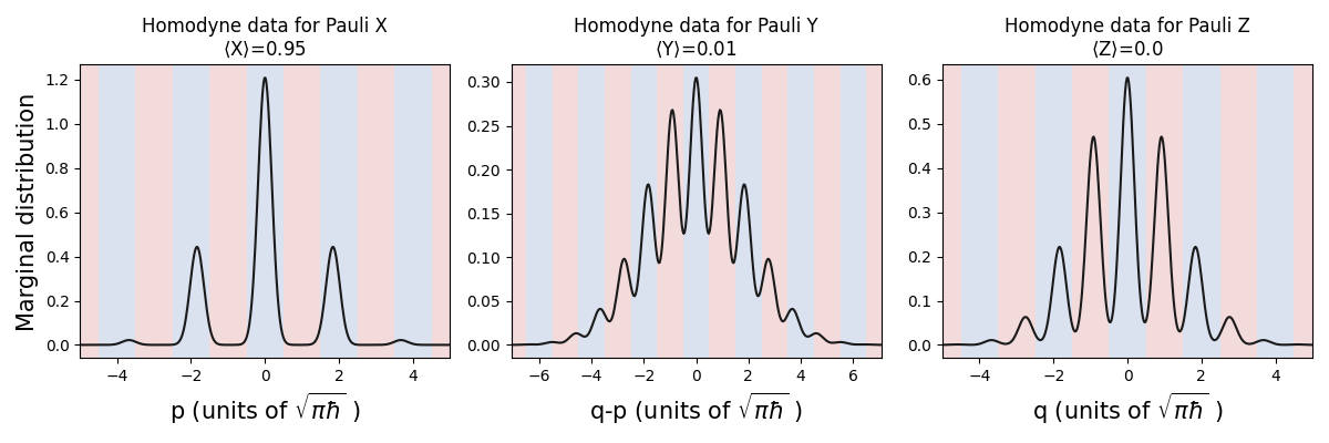
We see that the peaks in the homodyne distribution get broadened and shifted towards the origin, resulting in outcomes falling outside of the correct bins. This corresponds to qubit readout errors.
From this, we see the bosonic backend can be used to study noise and develop
strategies to deal with realistic effects on bosonic qubits.
Single-qubit Clifford gates
With Pauli measurements under our belt, we can move on to the single-qubit Clifford gates. As a summary, the association between GKP single-qubit Clifford gates and qubits is [6]:
Qubit gates |
CV gates |
|
|---|---|---|
Pauli X |
\(q\)-displacement by \(\sqrt{\pi\hbar}\) |
|
Pauli Z |
\(p\)-displacement by \(\sqrt{\pi\hbar}\) |
|
Hadamard |
Rotation by \(\pi/2\) |
|
Phase |
Quadratic phase gate of strength 1 |
We’ll demonstrate this mapping in the next few subsections.
Qubit Pauli X and Z gates: CV \(q\) and \(p\) displacements
The simplest examples are the qubit Pauli X
and Z gates,
which for the GKP encoding correspond to displacements
in phase space by \(\sqrt{\pi\hbar}\) along \(q\) and \(p\), respectively.
These can be implemented using the Xgate and Zgate operations.
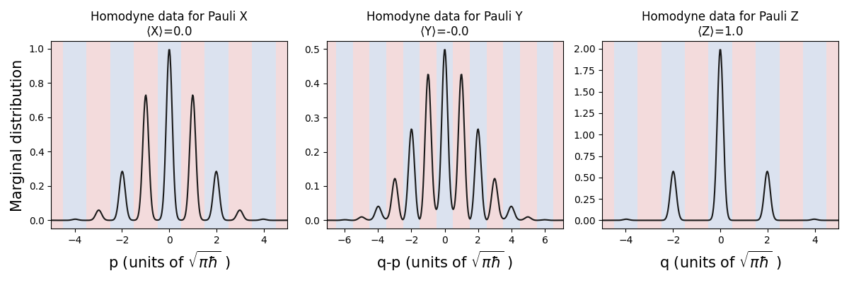
Below, we take a GKP qubit with \(\theta=\phi=np.pi/4\) and plot its marginal distributions along \(p\), \(q-p\), and \(q\) before and after applying a bit-phase flip. Recall that, once binned, this data provides the outcome of the Pauli measurements: blue (red) bins correspond to Pauli \(+1\) (\(-1\)) eigenvalues.
# Create a GKP state
prog = sf.Program(1)

with prog.context as q:
    sf.ops.GKP(state=[np.pi / 4, np.pi / 4], epsilon=0.08) | q

eng = sf.Engine("bosonic")
gkp = eng.run(prog).state

#Calculate and plot marginals
calc_and_plot_marginals(gkp, 0)
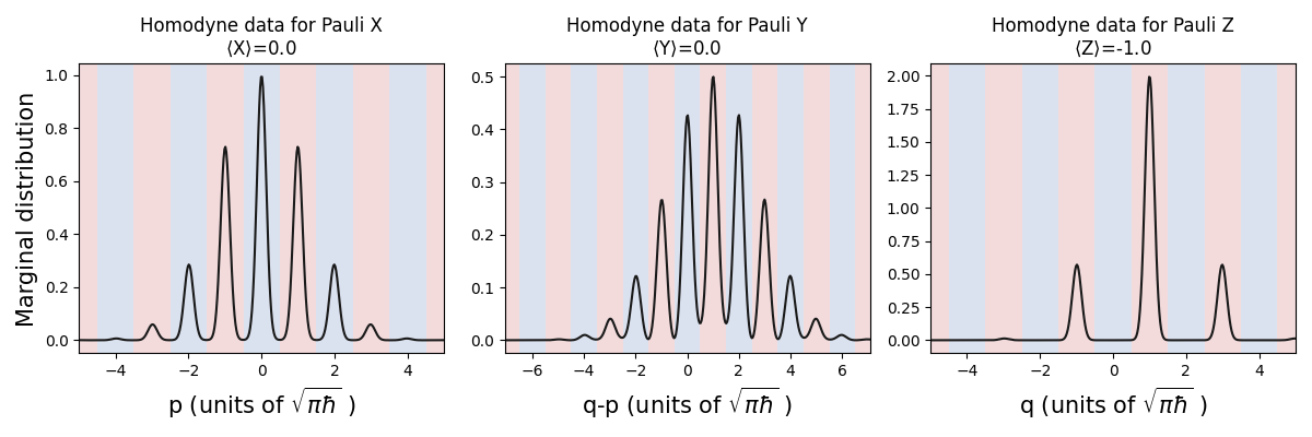
# Run it again but apply a bit-phase flip this time
prog = sf.Program(1)

with prog.context as q:
    sf.ops.GKP(state=[np.pi / 4, np.pi / 4], epsilon=0.08) | q
    sf.ops.Xgate(np.sqrt(np.pi * sf.hbar)) | q
    sf.ops.Zgate(np.sqrt(np.pi * sf.hbar)) | q

eng = sf.Engine("bosonic")
gkp = eng.run(prog).state

#Calculate and plot marginals
calc_and_plot_marginals(gkp, 0)
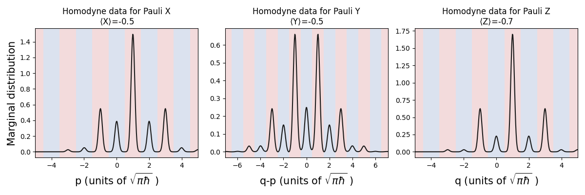
For \(p\) and \(q\) (associated with Pauli X and Z), we see that the regions of the distributions originally in the \(+1\) (blue) bins get shifted to \(-1\) (red) bins and vice versa. The distribution of \(q-p\) remains unchanged. This confirms the gates act as expected, since the probabilities of \(+1\) and \(-1\) outcomes from Pauli X and Z measurements get swapped by the bit-phase flip, while the Pauli Y is invariant!
Qubit Hadamard gate: CV rotation
The GKP Hadamard gate can be implemented by a \(\pi/2\) rotation in phase space. We’ve already indirectly seen this gate in action when toggling between different homodyne measurements. In the previous example, if a \(\pi/2\) rotation were applied to the state, the distribution of outcomes in \(q\) and \(p\) are interchanged, which means the the statistics of the Pauli X and Z outcomes are swapped as well, just as expected from a qubit Hadamard gate!
Qubit phase gate: CV quadratic phase gate
The GKP qubit phase
gate maps to the CV quadratic phase
gate, which can be implemented in Strawberry Fields with the existing
Pgate. This is a Gaussian operation, but unlike
rotations, the CV phase gate requires a squeezing operation.
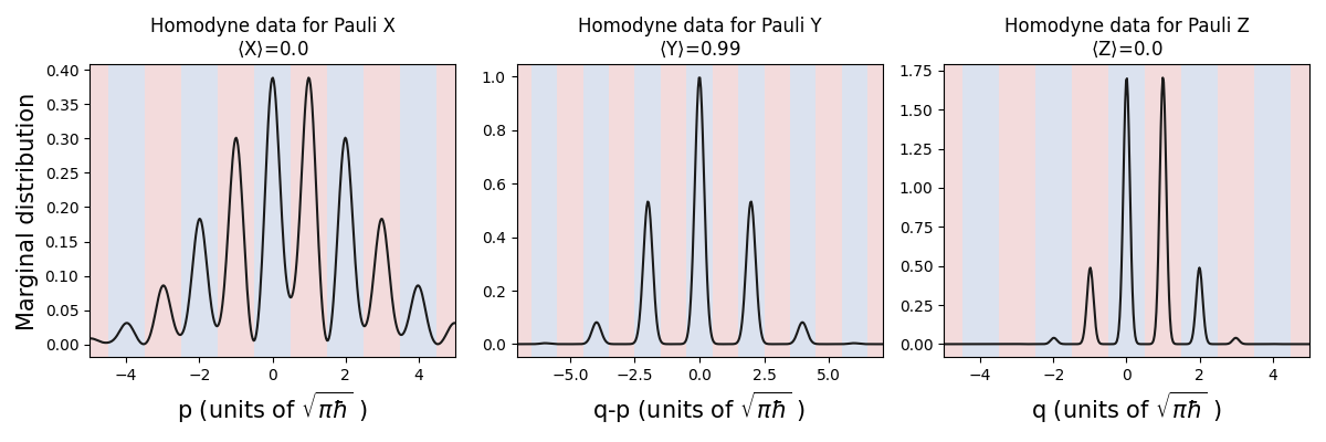
Let’s see the GKP phase gate in action on a qubit \(|+^\epsilon\rangle_{\rm gkp}\) state:
# Create a GKP |+> state and apply a phase gate
prog = sf.Program(1)

with prog.context as q:
    sf.ops.GKP(state=plus, epsilon=0.08) | q
    sf.ops.Pgate(1) | q

eng = sf.Engine("bosonic")
gkp = eng.run(prog).state

calc_and_plot_marginals(gkp, 0)
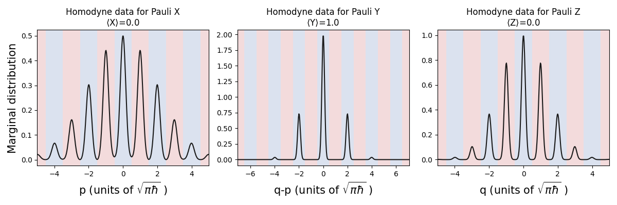
As expected, the homodyne outcomes associated with the Pauli Y measurement now fall entirely in the \(+1\) (blue) bins, reflecting that a standard qubit phase gate converts \(\hat{S}|+\rangle = |+i\rangle\).
As mentioned, the CV phase gate requires inline squeezing. In photonics, a feasible technique to do this is to apply measurement-based squeezing [7], which is essentially a method to teleport a squeezing operation onto a state. Briefly, the steps to do this are:
Interfere an ancillary squeezed vacuum state at a beamsplitter with the target state.
Perform a homodyne measurement on the ancillary mode.
Apply a feedforward displacement to the target mode based on the homodyne outcome.
The quality of measurement-based squeezing depends on the level of squeezing in the ancillary mode, and the efficiency of the homodyne detection.
While all backends of Strawberry Fields have implemented the ideal
inline squeezing operation through Sgate, to be able to study the
effects of realistic noise on bosonic qubits, for the bosonic
backend, we have also implemented measurement-based squeezing as
MSgate.
MSgate performs the teleportation circuit described above. The user
can specify whether they would like the map corresponding to the average
application of the teleportation circuit, or whether they want to
simulate a single-shot run and keep the homodyne sample on the ancillary
mode.
Below we examine how the quality of the GKP qubit phase gate changes once we replace the inline squeezing in the CV phase gate with measurement-based squeezing. We look first at the average map of the gate.
First, we define a phase gate that uses measurement-based squeezing.
r_anc and eta_anc are the level of squeezing and detection efficiency for
the ancilla. avg specifies whether to apply the average or single-shot map.
def MPgate(q, s, r_anc, eta_anc, avg):
    '''Applies a CV phase gate to a given mode using measurement-based squeezing.

    Args:
        q (object): label for the mode in the strawberryfields program
        s (float): the ideal phase gate parameter
        r_anc (float): level of squeezing in the ancillary mode
        eta_anc (0 <= float <= 1): detector efficiency for the ancillary mode
        avg (bool): True (False) applies the average (single-shot) mapping
    '''
    r = np.arccosh(np.sqrt(1 + s ** 2 / 4))
    theta = np.arctan(s / 2)
    phi = - np.pi / 2 * np.sign(s) - theta
    sf.ops.MSgate(r, phi, r_anc, eta_anc, avg) | q
    sf.ops.Rgate(theta) | q
Next, we create a GKP \(|+^\epsilon\rangle_{\rm gkp}\) state and apply a realistic phase gate (average map):
prog = sf.Program(1)

with prog.context as q:
    sf.ops.GKP(state=plus, epsilon=0.08) | q
    MPgate(q, 1, r_anc=1.2, eta_anc=0.95, avg=True)

eng = sf.Engine("bosonic")
gkp = eng.run(prog).state

calc_and_plot_marginals(gkp, 0)
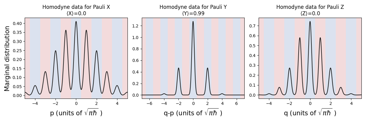
What happened? The peaks stayed essentially in the same places as in the previous simulation, but now they’ve become broader! Since more of each peak falls outside the correct bins, this will have an impact on likelihood of obtaining the correct Pauli measurement outcomes.
Let’s take a look at the single-shot implementation of the
measurement-based squeezing operation in the phase gate by setting avg to False:
prog = sf.Program(1)

with prog.context as q:
    sf.ops.GKP(state=plus, epsilon=0.08) | q
    MPgate(q, 1, r_anc=1.2, eta_anc=0.95, avg=False)

eng = sf.Engine("bosonic")
results = eng.run(prog)
gkp = results.state

calc_and_plot_marginals(gkp, 0)
On the face of it, these marginal distributions look very different! Luckily, the Pauli outcomes only depend on how much of the marginal distributions fall inside the correct bins, and less on the shapes and heights of the peaks within those bins. We notice that the homodyne distribution used for the Pauli Y measurement still falls primarily in the \(+1\) (blue) bins, although the peaks have broadened as compared to the ideal CV phase gate.
As promised, the homodyne outcome used for the feedforward operation can
be retrieved from the Results object output by the circuit:
print(results.ancillae_samples)
Out:
{0: [6.023905229521595]}
The dictionary key 0 denotes the mode where measurement-based
squeezing was applied, and the list entry contains the result of the
homodyne measurement on the ancillary state used in the feedforward
displacement of the measurement-based squeezing gate.
We’ve again seen through this example that the bosonic backend is
useful for studying realistic noise effects present in photonic circuits
applied to bosonic qubits. Next we move to two-qubit Clifford gates.
Two-qubit Clifford gates
Now that we understand single-qubit Clifford gates, we can move to two-qubit entangling gates. Another boon to the GKP encoding is the fact that certain two-qubit entangling gates such as the qubit CNOT and CZ gates correspond to deterministic Gaussian operations, specifically the CV CX and CZ gates:
Qubit gates |
CV gates |
|
|---|---|---|
CNOT |
CX gate of strength 1 |
|
CZ |
CZ gate of strength 1 |
As a simple demonstration of a two-qubit entangling gate, we apply a GKP CNOT gate on \(|+^\epsilon\rangle_{\rm gkp}\) and \(|0^\epsilon\rangle_{\rm gkp}\). For standard qubits, this yields the entangled state \(\frac{1}{\sqrt{2}}(|0,0\rangle+|1,1\rangle)\).
As a sanity check that this is indeed the state produced from the CNOT gate, we project the first qubit into the \(|0\rangle\) state by measuring \(q\)-homodyne (corresponding to a qubit Pauli Z measurment) and post-select on \(q_1=0\), which forces the outcome of the first mode into a \(+1\) (blue) bin. When we plot the marginal distribution of the second qubit after the measurement on the first qubit, we see that the distribution of \(q_2\) outcomes fall mainly into the \(+1\) (blue) bins, meaning the Pauli Z outcome on the second qubit will also be \(+1\), as expected.
Below, we create \(|+^\epsilon\rangle_{\rm gkp}\otimes|0^\epsilon\rangle_{\rm gkp}\) and apply a CNOT gate.
Then, we measure \(q\)-homodyne on the first mode, post-selecting on 0
via the select parameter:
prog = sf.Program(2)

with prog.context as q:
    sf.ops.GKP(state=plus, epsilon=0.1) | q[0]
    sf.ops.GKP(epsilon=0.1) | q[1]
    sf.ops.CXgate(1) | (q[0],q[1])
    sf.ops.MeasureHomodyne(0, select=0) | q[0]

eng = sf.Engine("bosonic")
gkp = eng.run(prog).state

calc_and_plot_marginals(gkp, 1)
We can do the same simulation, but this time postselect \(q_1=\sqrt{\pi\hbar}\), forcing the Pauli Z outcome of the first qubit to be \(-1\), since that value falls in a red bin. When we plot the marginal distributions of the second qubit, we see that the distribution of outcomes in \(q_2\) now fall in the \(-1\) (red) bins, indicating the correct qubit state was created by the two-qubit gate.
prog = sf.Program(2)

with prog.context as q:
    sf.ops.GKP(state=plus, epsilon=0.1) | q[0]
    sf.ops.GKP(epsilon=0.1) | q[1]
    sf.ops.CXgate(1) | (q[0],q[1])
    sf.ops.MeasureHomodyne(0, select=np.sqrt(np.pi * sf.hbar)) | q[0]

eng = sf.Engine("bosonic")
gkp = eng.run(prog).state

calc_and_plot_marginals(gkp, 1)
The CV CX
gate used to implement the GKP qubit CNOT gate requires
beamsplitters, rotations and inline squeezing.
While we did not examine it here, the same realistic
noise effects we examined for the other operations – be it loss or
measurement-based squeezing – could be simulated for two qubit gates
using the bosonic backend.
Non-Clifford T gate
To complete the set of universal gates for GKP qubits, we need one non-Clifford gate. As it turns out, the GKP qubit T gate can be applied through gate teleportation by using an ancillary GKP qubit magic state (a non-Pauli eigenstate) and Gaussian operations [2].
The steps to apply the T gate build on all the previous examples we’ve seen:
Entangle the ancillary magic state and the data state with a qubit CNOT gate, i.e. a CV CX gate.
Perform a Pauli Z measurement on the ancillary mode via a binned CV \(q\)-homodyne measurement.
Based on the outcome of the Pauli measurement, apply a feedforward qubit phase gate (a CV phase gate) to the data mode.
Ideally, the GKP qubit magic state one would use is given by \(|M\rangle_{\rm gkp}=\frac{1}{\sqrt{2}}(e^{-i\pi/8}|0\rangle_{\rm gkp} + e^{i\pi/8}|1\rangle_{\rm gkp})\). Next, we will see the effect of using a finite-energy GKP \(|M^{\epsilon}\rangle_{\rm gkp}\) for gate teleportation.
We apply the qubit T gate to the state \(|M^{\epsilon}\rangle_{\rm gkp}\) itself, knowing that for standard qubits \(\hat{T}|M\rangle=|+i\rangle\). For this simulation, we will postselect on a homodyne outcome for the ancillary mode that will cause the feedforward phase gate to be applied.
# Define a binning function to get the Pauli Z outcome for the feedforward
def gkp_binning(x):
    '''Bins a homodyne outcome to a binary 0 or 1 according to the GKP bin structure.
    Pauli +1 (-1) corresponds to 0 (1).

    Args:
        x (float): homodyne outcome value
    '''
    term_1 = (x + np.sqrt(np.pi) / 2) / np.sqrt(4 * np.pi)
    term_2 = (x + np.sqrt(np.pi) / 2) // np.sqrt(4 * np.pi)
    return (term_1 - term_2) // 0.5

# Create GKP magic states and perform the T gate teleportation circuit
magic = [np.pi / 2, - np.pi / 4]
prog = sf.Program(2)

with prog.context as q:
    sf.ops.GKP(state=magic, epsilon = 0.1) | q[0]
    sf.ops.GKP(state=magic, epsilon = 0.1) | q[1]
    sf.ops.CXgate(1) | (q[0], q[1])
    sf.ops.MeasureHomodyne(0, select=np.sqrt(np.pi * sf.hbar)) | q[1]
    sf.ops.Pgate(gkp_binning(q[1].par)) | q[0]

eng = sf.Engine("bosonic")
gkp = eng.run(prog).state

calc_and_plot_marginals(gkp, 0)
We find that the output homodyne distributions match what we expect for the \(|+i\rangle\) qubit state: the distribution along \(q-p\) falls mainly within \(+1\) (blue) bins, while the other quadratures fall evenly between red and blue bins.
An interesting effect to note is that the peaks are broader in some
quadratures than others. This demonstrates that through the gate
teleportation process, the data qubit picked up some of the
finite-energy noise from the ancillary magic state. These types of realistic
effects are easy to study using the bosonic backend!
Conclusion
In this tutorial, we showed the translation between the universal set of
GKP qubit gates and their CV Gaussian phase space implementations. We
performed simulations using the bosonic backend, a tool specialized to
study how bosonic qubits transform under the types of Gaussian
transformations and measurements necessary for the GKP encoding.
References and Footnotes
- 1(1,2,3)
J. Eli Bourassa, Nicolás Quesada, Ilan Tzitrin, Antal Száva, Theodor Isacsson, Josh Izaac, Krishna Kumar Sabapathy, Guillaume Dauphinais, and Ish Dhand. Fast simulation of bosonic qubits via Gaussian functions in phase space. arXiv:2103.05530, 2021.
- 2(1,2,3,4)
Daniel Gottesman, Alexei Kitaev, and John Preskill. Encoding a qubit in an oscillator. doi:10.1103/PhysRevA.64.012310.
- 3
For the advanced reader: when we call
sf.ops.GKP(), we are still only creating a finite-energy GKP state. However, the locations of peaks in that state are close enough to the ideal state, and the signs of the weights match the ideal state, so we can use it for a pedagogical illustration of the ideal GKP states.- 4
L. García-Álvarez, A. Ferraro, and G. Ferrini. From the Bloch Sphere to Phase-Space Representations with the Gottesman-Kitaev-Preskill Encoding. doi:10.1007/978-981-15-5191-8_9.
- 5
Ben Q. Baragiola, Giacomo Pantaleoni, Rafael N. Alexander, Angela Karanjai, and Nicolas C. Menicucci. All-Gaussian Universality and Fault Tolerance with the Gottesman-Kitaev-Preskill Code. doi:10.1103/PhysRevLett.123.200502.
- 6
A note for the keen reader: An extra advantage of the GKP encoding is that there is in fact a one-to-many mapping of qubit to CV gates. Taking Pauli gates as an exmaple, a displacement by any odd multiple of \(\sqrt{\pi\hbar}\) along \(q\) (\(p\)) will effect a Pauli X (Z) gate. The direction of displacements can be varied in the circuit compilation to avoid too much energy being injected into the state, which would happen if the displacements were always in the same direction.
- 7
Radim Filip, Petr Marek, and Ulrik L. Andersen. Measurement-induced continuous-variable quantum interactions. doi:10.1103/PhysRevA.71.042308.
Total running time of the script: ( 1 minutes 48.877 seconds)
Contents
Downloads
Related tutorials