Gaussian cloning

“The natural generalization of teleportation to the many-recipient case” — van Loock [1]

A fundamental concept in quantum mechanics, the no-cloning theorem states that an unknown quantum state cannot be copied exactly [2] - in effect, ruling out any algorithm that attempts to produce or relies upon the production of perfect copies of an arbitrary quantum state [3]. Nevertheless, the no-cloning theorem does not rule out the production of approximate quantum state clones. This has led to the development of so called ‘quantum cloning algorithms’, unitary cloning transformations which provide identical copies of an arbitrary input state, at the cost of a non-unity fidelity.

Implementation

The first approximate cloning algorithm was introduced in the context of discrete-variable quantum computing by Buzek and Hillery [4], and quickly followed up with a CV implementation by Cerf et al. [5]. Here, a class of cloning machines satisfying displacement covariance are introduced; that is, for two input states \(\ket{\psi}\) and \(\ket{\phi}\), with approximate cloned states \(\ket{\psi'}\) and \(\ket{\phi'}\) respectively,

\[D(\alpha)\ket{\psi}=\ket{\phi}~~~\Rightarrow~~~D(\alpha)\ket{\psi'}=\ket{\phi'}\]

In other words, cloning fidelity is invariant under displacements in the phase space, and the position and momentum uncertainties of the two clones satisfies the uncertainty inequality

\[\Delta x_1\Delta p_2 \geq \frac{1}{2}\hbar\]

where \(\Delta x_1\) is the \(x\) quadrature variance of state \(\ket{\psi}\) and \(\Delta p_2\) is the \(p\) quadrature variance of state \(\ket{\phi}\).

Gaussian cloning algorithms, those with the ability to produce two approximate and identical clones of the input state with theoretically optimum fidelity, are a subclass of the displacement covariant cloners that also exhibit rotational covariance. As a result, Gaussian cloning fidelity is invariant under both displacement and rotation in the phase space, and the resulting cloned states have identical \(x\) and \(p\) quadrature variances, \(\Delta x_1=\Delta p_1=\Delta x_2=\Delta p_2\). It is this subclass which is shown to be the CV equivalent to the universal qubit cloner of Buzek and Hillery [5].

Circuit analysis

Working within this framework, Andersen et al. [6] presented a symmetric Gaussian cloning algorithm (in addition to experimental results) for optimum theoretical cloning of coherent states:

Here, \(\ket{\alpha_0}\) represents an input coherent state, \(\ket{\alpha'}_1\) and \(\ket{\alpha'}_3\) represent the two identical but approximate clones, and the beamsplitters are 50-50 beamsplitters (hence the ‘symmetric’ in symmetric cloning algorithm). Let’s walk through the various stages of the circuit above, and examine what is occuring.

1. The action of a 50-50 beamsplitter on a coherent state \(\ket{\alpha}\) and a vacuum state \(\ket{0}\) is \(BS(\ket{\alpha}\otimes\ket{0}) = \ket{\frac{1}{\sqrt{2}}\alpha}\otimes \ket{\frac{1}{\sqrt{2}}\alpha}\). As such, after the two beamsplitters, the circuit exists in the following state:

   \[\ket{\frac{1}{\sqrt{2}}\alpha_0}\otimes \ket{\frac{1}{2}\alpha_0}\otimes \ket{\frac{1}{2}\alpha_0}.\]

2. Performing the homodyne detection on modes \(q_1\) and \(q_2\) results in the two normally distributed measurement variables \(u\) and \(v\) respectively:

   \[u\sim N\left(\sqrt{\frac{\hbar}{2}}\text{Re}(\alpha_0), \frac{\hbar}{2}\right), ~~~ v\sim N\left(\sqrt{\frac{\hbar}{2}}\text{Im}(\alpha_0), \frac{\hbar}{2}\right).\]

3. Two controlled displacements \(X(\sqrt{2}u)=D(u/\sqrt{\hbar})\) and \(Z(\sqrt{2}v)=D(iv/\sqrt{\hbar})\) are then performed on mode \(q_0\):

   \[D\left(\frac{1}{\sqrt{\hbar}}(u+iv)\right)\ket{\frac{1}{\sqrt{2}}\alpha_0} = \ket{\frac{1}{\sqrt{2}}\alpha_0 + \frac{1}{\sqrt{\hbar}}(u+iv)} = \ket{\tilde{\alpha_0}}\]

   Since we are displacing a coherent state, the result of the controlled displacements remains a pure coherent state. However, since the parameters of the controlled displacements are themselves random variables, we must describe the resulting coherent state by a rando variable \(\tilde{\alpha_0} \sim N(\mu, \text{cov})\).

   Here, \(\tilde{\alpha_0}\) is randomly distributed as per a multivariate normal distribution with vector of means \(\mu=\sqrt{2}(\text{Re}(\alpha_0), \text{Im}(\alpha_0))\) and covariance matrix \(\text{cov}=\I/2\).

4. Finally, we apply another beamsplitter to mode \(q_0\) and mode \(q_3\) in the vacuum state, to get our two cloned outputs:

   \[BS(\ket{\tilde{\alpha_0}}\otimes\ket{0}) = \ket{\frac{1}{\sqrt{2}}\tilde{\alpha_0}}\otimes \ket{\frac{1}{\sqrt{2}}\tilde{\alpha_0}} = \ket{\alpha'}\otimes \ket{\alpha'}.\]

   where \(\alpha' \sim N(\mu, \text{cov}), ~~\mu=(\text{Re}(\alpha_0), \text{Im}(\alpha_0)), ~~\text{cov}=\I/4\).

Coherent average fidelity

If we were to perform the Guassian cloning circuit over an ensemble of identical input states \(\ket{\alpha_0}\), the cloned output can be described by the following mixed state,

\[\rho = \iint d^2 \alpha' \frac{2}{\pi}e^{-2|\alpha'-\alpha_0|^2}\ket{\alpha'}\bra{\alpha'},\]

where the exponential term is the PDF of the random variable \(\alpha'\) from (4) above. To calculate the average fidelity over the ensemble of the cloned states, it is sufficient to calculate the inner product

\[F = \braketT{\alpha_0}{\rho}{\alpha_0}.\]

From the Fock basis decomposition of the coherent state (see Coherent state), it can be easily seen that \(|\braketD{\alpha_0}{\alpha'}|^2 = e^{-|\alpha_0-\alpha'|^2}\). Therefore,

\[F = \frac{2}{\pi}\iint d^2 \alpha' e^{-2|\alpha'-\alpha_0|^2} |\braketD{\alpha_0}{\alpha'}|^2 = \frac{2}{\pi}\iint d^2 \alpha ~e^{-3|\alpha|^2} = \frac{2}{3},\]

where we have made the substitution \(\alpha=\alpha'-\alpha_0\). Note that the average fidelity is independent of the initial state \(\alpha_0\).

Note

The above is calculated in the case of unity quantum efficiency \(\eta=1\). When \(\eta<1\), there is non-zero uncertainty in the homodyne measurement, \(\sigma_H=\frac{1-\eta}{\eta}\), and in practice the symmetric Gaussian cloning scheme has coherent state average cloning fidelity given by

\[F(\sigma_H)=\frac{2}{3+\sigma_H}\]

In the case of the Gaussian backend, \(\sigma_H=2\times 10^{-4}\) (see GaussianBackend.measure_homodyne).

Displaced squeezed states

In addition to coherent states, this cloning scheme was further analysed by Olivares et al. [7] in the cases of other Gaussian input states, such as squeezed states and thermal states. In particular, when the input Gaussian state is a displaced squeezed state,

\[\ket{\psi} = \ket{\alpha,z} = D(\alpha)S(z)\ket{0},\]

this scheme provides an optimum fidelity of \(2/3\) only if the squeezing parameter is known beforehand, as this allows the application of the unitary operation \(S(z)^{-1}\) to recover a coherent state prior to cloning. Of course, this is not possible if we wish to clone an arbitrary unknown displaced squeezed state; in this case, the scheme described above leads to the following fidelity:

\[F(r,\sigma_H) = \frac{4}{\sqrt{(6+2\sigma_H)^2+32(1+\sigma_H)\sinh^2(r)}}\]

where \(z=re^{i\phi}\) and \(\sigma_H\) is the uncertainty in the homodyne measurement. Note that \(F\rightarrow0\) as \(r\rightarrow\infty\); i.e., the more highly squeezed the state, the lower the cloning fidelity.

Code

The symmetric Gaussian cloning circuit displayed above can be implemented using Strawberry Fields:

import strawberryfields as sf
from strawberryfields.ops import *
from numpy import pi, sqrt
import numpy as np

gaussian_cloning = sf.Program(4)

with gaussian_cloning.context as q:
    # state to be cloned
    alpha = 0.7+1.2j
    Coherent(np.abs(alpha), np.angle(alpha)) | q[0]

    # 50-50 beamsplitter
    BS = BSgate(pi/4, 0)

    # symmetric Gaussian cloning scheme
    BS | (q[0], q[1])
    BS | (q[1], q[2])
    MeasureX | q[1]
    MeasureP | q[2]
    Xgate(q[1].par * sqrt(2)) | q[0]
    Zgate(q[2].par * sqrt(2)) | q[0]

    # after the final beamsplitter, modes q[0] and q[3]
    # will contain identical approximate clones of the
    # initial state Coherent(0.1+0j)
    BS | (q[0], q[3])

Since all operations and measurements are Gaussian, we can use the Gaussian backend:

eng = sf.Engine(backend="gaussian")

Modes 1 and 2 are ancilla modes; we are interested in extracting modes 0 and 3.

results = eng.run(gaussian_cloning, modes=[0, 3])

After constructing the circuit and running the engine, we can call the state method fidelity_coherent() to calculate the fidelity of the two cloned output states compared to the input coherent state \(\alpha=0.7+1.2j\).

Note that we take the square root since the method is returning the fidelity of both modes multiplied.

fidelity = sqrt(results.state.fidelity_coherent([0.7+1.2j, 0.7+1.2j]))
print(fidelity)

Out:

0.5572817882335409

While fidelity_coherent is supported by both the Gaussian and the Fock backends, the 'gaussian' backend additionally supports extracting the mean displacement of output states, using displacement():

alpha = results.state.displacement()

Checking that they are identical clones up to numerical error:

print(alpha[0] - alpha[1] <= 1e-15)

Out:

True

In order to calculate the average fidelity over an ensemble, we will need to run the circuit multiple times, and calculate the mean fidelity over all runs:

# run the engine over an ensemble
reps = 1000
f = np.empty([reps])
a = np.empty([reps], dtype=np.complex128)

for i in range(reps):
    eng.reset()
    results = eng.run(gaussian_cloning, modes=[0])
    f[i] = results.state.fidelity_coherent([0.7+1.2j])
    a[i] = results.state.displacement()

print("Fidelity of cloned state:", np.mean(f))
print("Mean displacement of cloned state:", np.mean(a))
print("Mean covariance matrix of cloned state:", np.cov([a.real, a.imag]))

Out:

Fidelity of cloned state: 0.6598662763090357
Mean displacement of cloned state: (0.7124677707668282+1.2145178434535502j)
Mean covariance matrix of cloned state: [[0.25597159 0.00122702]
 [0.00122702 0.25298511]]

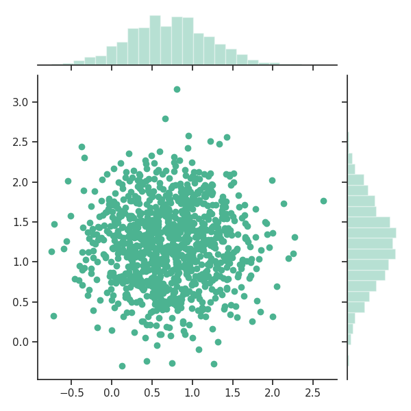
Plotting the scatter plot of a.real vs. a.imag, we see that they are indeed distributed as a multivariate normal distribution, with a mean of \(\sim 0.7+1.2j\), and covariance \(\sim I/4\):

import seaborn as sns
sns.set(style="ticks")
sns.jointplot(a.real, a.imag, color="#4CB391")

Out:

<seaborn.axisgrid.JointGrid object at 0x7faec1f23110>

References

1

P. van Loock and Samuel L. Braunstein. Telecloning of continuous quantum variables. Physical Review Letters, Nov 2001. doi:10.1103/physrevlett.87.247901.

2

W. K. Wootters and W. H. Zurek. A single quantum cannot be cloned. Nature, 299(5886):802–803, Oct 1982. doi:10.1038/299802a0.

3

D. Dieks. Communication by EPR devices. Physics Letters A, 92(6):271–272, Nov 1982. doi:10.1016/0375-9601(82)90084-6.

4

V. Bužek and M. Hillery. Quantum copying: beyond the no-cloning theorem. Physical Review A, 54(3):1844–1852, Sep 1996. doi:10.1103/physreva.54.1844.

5(1,2)

N. J. Cerf, A. Ipe, and X. Rottenberg. Cloning of continuous quantum variables. Physical Review Letters, 85(8):1754–1757, Aug 2000. doi:10.1103/physrevlett.85.1754.

6

Ulrik L. Andersen, Vincent Josse, and Gerd Leuchs. Unconditional quantum cloning of coherent states with linear optics. Physical Review Letters, Jun 2005. doi:10.1103/physrevlett.94.240503.

7

Stefano Olivares, Matteo G. A. Paris, and Ulrik L. Andersen. Cloning of gaussian states by linear optics. Physical Review A, Jun 2006. doi:10.1103/physreva.73.062330.

demos/run_gaussian_cloning

 

Download Python script

 

Download Notebook